The Hebb's learning rule module
In this paragraph we introduce the Hebb's learning rule models, which are an example of unsupervised learning algorithms.
In INNE we implemented three models of unsupervised learning algorithms: Hebbian models
with different learning rules, simple competitive learning
and the Kohonen feature map.
The panel to
drive the simulation will open when the item HEBBIAN MODEL in the MODEL sub-menu is choosen.
The Hebb's model: an overview
The Hebbian unsupervised algorithms are based
on a law specified by Donald Hebb
[Hebb 1949] in 1949,
studying the cellular modifications that occur in animals while learning. He
observed that the connection between two neurons are strengthened when both
neurons are active simultaneously.
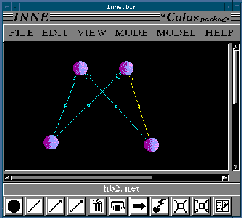
The networks are linear and a typical architecture is
shown in this figure.
The ith output Oi is given by:

where wi is the weight vector for the ith output; the input
vectors I are N-dimensional, they hold continuos or
binary values with mean = 0.
The learning rules that we have implemented in the Hebbian module are:
- the plain Hebbian rule;
- the Oja rule;
- the Sanger rule.
The plain Hebbian rule is usable only in the case of a single
linear output unit and it is governed by the follow equation:

where eta controls the learning rate.
This strengthens the output in turn for each input presented, so
frequent input patterns will have most influence in the long run,
and will come to produce the largest output. But there is a
problem: the weights keep on growing without bound and
learning never stops; infact, the direction with the largest
eigenvalue  of C (the correlation matrix) would
eventually become dominant, so that w would gradually
approach an eigenvector corresponding to
  , with
a increasing huge norm.
We have prevented the divergence of this rule by constraining
the growth of the weight vector w; we have used a simple
renormalization wi’= wi/|w of all the weights after each
update.
Oja in 1982 suggested a more clever approach; he showed that
it is possible to make the weight vector approach a constant
length without having to do any normalisation.
Oja'’s rule corresponds to adding a weight decay proportional to
 to the plain Hebbian rule:

where delta w depends on the difference between the actual
input and the back-propagated output.
Oja’'s rule converges to a weight vector w with the following
properties:
- unit length: |w|=1;
- eigenvector direction: w lies in a maximal eigenvector
direction of C;
- variance maximization: w lies in the direction that maximize
 .
.
This rule is useful for one-output network, it would however be
desiderable to have M-output network that extract the first M
principal components. Oja and Sanger
[Sanger 1989] have both
designed one-layer feed-forward networks that do this; the
Oja'’s M unit rule is:

and the Sanger'’s rule (Generalized Hebbian Algorithm) is:

the only difference is in the upper limit of the summation and
both rules reduce to Oja’'s one-output rule.
For Oja'’s M-unit rule the M weight vector converge to span the
same subspace as these first M eigenvectors, but do not find the
eigenvector direction themselves. It gives weight vectors which
differ from trial to trial and spanning the right subspace; they
depend on the initial condition and on the particular data
samples seen during learning. On average the variance of each
output is the same and this may be useful in some applications
where one wants to keep the information spread uniformly
across the units. Furthermore, if any algorithm of this sort is
implemented in real brains, it would look more like Oja's than
Sanger'’s rule
The Sanger'’s rule extracts the principal components in order; it
performs exactly the Karhunen_Loe’ve transform. The
Generalized Hebbian Algorithm was designed combining the
Oja’'s one-unit rule and the Gram-Schmidt orhtogonalization
process.
Sanger
[Sanger 1989] has proved the following:
Theorem: If W(the matrix weight vector) is assigned random
weight at time zero,  and
and  ; then with
probability 1, the Generalized Hebbian Algorithm will
converge, and W will approach the matrix whose rows are the
first M eigenvectors of the input correlation matrix C,
ordered by decreasing eigenvalue.

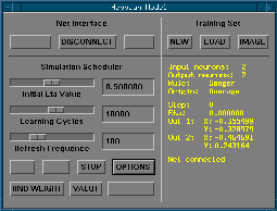
The panel to drive the simulation
with its option panel allowing to select the learning rule.
Reference
- T.D. Sanger (1989)
- Optimal Unsupervised Learning in a Single-Layer Linera feedforward Neural Network. Neural Networks, 2:459-473
- D. O. Hebb (1949)
- The organization of behaviour. In J.A. Anderson and E. Rosenfeld (eds) Neuro Computing, 1988
 Back to index


 of C (the correlation matrix) would
eventually become dominant, so that w would gradually
approach an eigenvector corresponding to
  to the plain Hebbian rule:
 .
.


 and
and  ; then with
probability 1, the Generalized Hebbian Algorithm will
converge, and W will approach the matrix whose rows are the
first M eigenvectors of the input correlation matrix C,
ordered by decreasing eigenvalue.

 Back to index